Databricks Free Edition with dbt Core

I traded e-mails with a colleague working through issues configuring dbt for use with their new Databricks Free Edition workspace. For others working through similar issues, this post is a summation of the set up instructions I shared and links for further reading.

Set Up Instructions

Databricks announced a new free edition of the their data platform in June 2025 intended for learners and hobbyists. Data engineers and analysts can use dbt with Databricks Free Edition.

Configuring Databricks

  1. Login to your Databricks Free Edition account by navigating to https://login.databricks.com/.
  2. Sign-up for an account or sign-in if you have an existing account.
  3. Create a new personal access token (PAT).
    • Select Settings from the user menu at the top right of the page.
    • Click the Developer link under the User section of the Settings menu.
    • Click Manage to the right of the Access Tokens header.
    • Click the Generate new token button.
  4. Save the token in a secure place for later use.
  5. Select Catalog from the menu bar on the left side of the page.
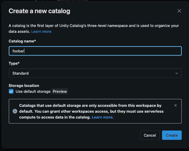
  6. Click the + sign to the top right of the Catalog pane.
  7. Enter the name of the catalog in the Catalog name* field.
  8. Ensure the Type* drop has “Standard” selected.
  9. Ensure the Use default storage is checked.
  10. Click the Create button.

    Databricks Create New Catalog Modal
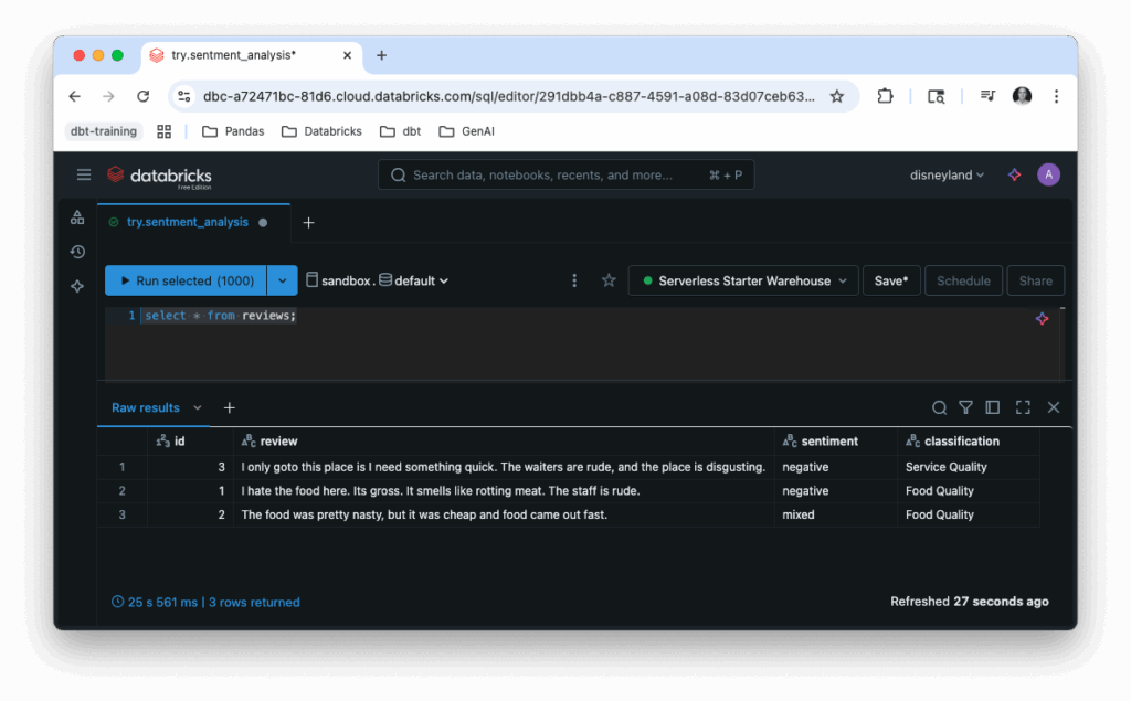
  11. Select SQL Warehouse from the menu bar on the left side of the page.
  12. Click the “Serverless Starter Warehouse” link on the Compute page.
  13. Click the Start button at the top right of the page.
  14. Save the URL for later use.

Configuring dbt

The instructions in this post were run on machines with the following software versions:

  • MacOS 15.5
  • Bash 3.2.57
  • Python 3.13.5
  • dbt Core 1.10.5
  • dbt Databricks plugin 1.10.4

I used the following steps to configure dbt Core.

  1. Open a new terminal.
  2. Confirm Python 3.7 or greater is available on your system. I am using Python 3.13.5.
  3. Create a new directory.
  4. Navigate to the directory.
  5. Create a new virtual environment: python -m venv env
  6. Activate the virtual environment: source ./env/bin/activate
  7. Install the dbt-core and dbt-databricks packages:
    python -m pip install dbt-core dbt-databricks
  8. Initialize your new Databricks project
    • Run dbt init from the commandline
    • Provide the information when prompted.
      • When asked “Which database would you like to use?”, choose “databricks”.
      • When asked “host (yourorg.databricks.com)”, choose the subdomain and domain portion of the SQL warehouse URL e.g., dbc-b82471fc-21d3.cloud.databricks.com
      • When asked “http_path (HTTP Path)”, provided the path portion of the SQL warehouse URL e.g., /sql/warehouses/723b706a90da12d4
      • When asked “Desired access token option (enter a number)”, select “use access token”.
      • When asked “token (dapiXXXXXXXXXXXXXXXXXXXXXXXXXXXXXXXX)”, paste the PAT you generated.
      • When asked “Desired unity catalog option (enter a number)”, select “use Unity Catalog”.
      • When asked “catalog (initial catalog)”, enter the name of your catalog.
      • When asked “schema (default schema that dbt will build objects in)”, enter “default”.
      • When asked “threads (1 or more) [1]”, choose the right number of threads for your application. I choose 1 thread for my project.
  9. Navigate into the project folder.
  10. Run the debug to verify you environment has bee set up successfully: dbt debug

Additional Resources

5-Minute Sentiment Analysis with Databricks

Alex Lichen and Ina Felsheim wrote a blog titled “Step-by-Step Guide: AI-Powered Customer Sentiment Analysis” that described how to perform sentiment analysis with Databricks SQL’s AI Functions such as ai_analyze_sentiment and ai_classify. I think the article is brilliant and serves as a great vehicle to explain how to develop this use case on the platform. While most of the customers I work with are interested in using these capabilities to address their sentiment analysis workloads, the article didn’t really resonate with managers and less technical audiences. I found that this audience rarely read the full article on follow-up.

I created a quick demonstration based on the article that takes about 5 minutes to run and present. The demo consists of a single notebook that creates a table, populates it with sample reviews, and performs analysis on those reviews. Its intended to be absurdly short and painfully simple.

You can find the code for this demo in the adamfortuno/Try.Databricks.Sentiment-Analysis repository. The magic is in the try.sentiment_analysis.ipynb notebook, though I’ll cover the key components here.

Setup and Table Creation

I’ve deployed this notebook in a Databricks Free Edition workspace. My workspace has a catalog named sandbox containing two schema: default and information_schema. I use the default schema for this demo.

We’re going to create a reviews table in the sandbox database’s default schema:

DROP TABLE IF EXISTS sandbox.default.reviews;

CREATE TABLE sandbox.default.reviews (
  id int primary key
, review string
, sentiment string
, classification string
);

We’re storing the review text, sentiment, and a category. The “review” is the customer’s feedback. Sentiment indicates the consumer’s general satisfaction: positive, negative, or mixed. The “classification” identifies the primary subject of the consumer’s review. For example, a quick-service restaurant might have review categories like price, store cleanliness, taste, and service.

Insert Consumer Reviews

We’ll add some fictional customer reviews to the reviews table leaving the sentiment and classification fields null as those values will be derived later.

INSERT INTO sandbox.default.reviews (id, review)
VALUES (1, "I hate the food here. Its gross. It smells like rotting meat. The staff is rude.");

INSERT INTO sandbox.default.reviews (id, review)
VALUES (2, "The food was pretty nasty, but it was cheap and food came out fast.");

INSERT INTO sandbox.default.reviews (id, review)
VALUES (3, "I only goto this place is I need something quick. The waiters are rude, and the place is disgusting.");

Consumer Review Analysis

We’re going to analyze these consumer reviews to derive sentiment and focus area. This would help our restaurant identify areas for improvement. We have the sentiment analysis and review category derived in separate cells.

--Derive sentiment
MERGE INTO sandbox.default.reviews AS trg
USING (
  SELECT id
       , review
       , ai_analyze_sentiment(review) as sentiment
  FROM sandbox.default.reviews
) AS src
ON trg.id = src.id
WHEN MATCHED THEN
  UPDATE SET sentiment = src.sentiment;

SELECT * FROM sandbox.default.reviews;

The ability to assess sentiment with a single function — ai_analyze_sentiment() — is the definition of simplicity. This eliminates a ton of code around chunking and vectorizing your reviews before submission to an LLM for analysis.

Next, we’ll use the ai_classify function to determine the focus of the review. We’re passing the review as well as an array of classification categories.

MERGE INTO sandbox.default.reviews AS trg
USING (
  SELECT id
       , review
       , ai_classify(review, ARRAY('Food Quality', 'Service Quality', 'Location Quality')) as classification
  FROM sandbox.default.reviews
) AS src
ON trg.id = src.id
WHEN MATCHED THEN
  UPDATE SET classification = src.classification;

SELECT * FROM sandbox.default.reviews;

In this case, I’ve stored the sentiment and classification category with each review. While there are several ways to model this data depending on your specific use case, I’ve kept it intentionally .

Query reviews table

Finally, I create a bar chart to visualize the results:

%python
import plotly.express as px
import pandas as pd

review_table = "sandbox.default.reviews"

sdf = spark.table(review_table)
pdf = sdf.toPandas()

# Count reviews by classification
classification_counts = pdf['classification'].value_counts()

# Create bar chart
fig = px.bar(
    x=classification_counts.index,
    y=classification_counts.values,
    title='Number of Reviews by Classification',
    labels={'x': 'Classification', 'y': 'Number of Reviews'}
)

fig.show()

This simple bar chart compares the number of reviews by category.

While I could demonstrate this using an AI/BI Dashboard or show how to analyze this data using natural language with AI/BI Genie, a Plotly dashboard directly in the demo notebook keeps the focus on the ease of generating sentiment and classification insights.

Feel free to use this demo to showcase Databricks’ new AI functions with colleagues and coworkers. The 5-minute format makes it accessible to both technical and non-technical audiences while demonstrating the power and simplicity of Databricks’ AI capabilities.

Levenshtein Distance and Distance Similarity Functions

Russian scientist Vladimir Levenshtein discovered the Levenshtein Distance algorithm in 1965. The algorithm produces the number of edits (i.e., insertions, deletions, and substitutions) required to change one string into the other. Consider the distance between “Steven” and “Stephen”:

Step-1: Substitute "v" for "p"
Step-2: Insert "h" after the "p"

It takes two edits to change “Steven” to “Stephen”. The distance is 2.

The distance similarity expands on the distance algorithm by creating a percentage from the number of edits (distance algorithm’s output). The percentage indicates how similar the words are to one another. We needed two edits to change Steven to Stephen in the example above. That could be expressed by saying Steven is 71% similar to Stephen.

It’s calculated with the following formulae:

[distance_similarity] = 100 - ([distance] / [length_of_longest_string] * 100)

Apache Spark includes an implementation of the Levenschtein Distance function. To implement the distance similarity, your code needs to perform the extra calculations:

## Import the `levenshtein` function
from pyspark.sql.functions import levenshtein

## Creating a single data from with the values I want to compare
df0 = spark.createDataFrame([('kitten', 'sitting',)], ['l', 'r'])

## Let's compare the two values...
df0.select(levenshtein('l', 'r').alias('d')).collect()

The following list of name pairs can be enriched to provide their distance similarity.

foo,bar
Suzie Chappman,Suzy Chappman
Billy Wonka,William Wonka
Kelly Schmitt,Kelly Schmitt
Devon Parker,Devon Jones
Kylie LeBlanc,Stacy LeBow

In the following, we use PySpark to establish the similarity between each pair of names:

from pyspark.sql import SparkSession
from pyspark.sql.functions import levenshtein, length, when, col
from pyspark.sql.types import IntegerType

def spark_session_get():
    try:
        spark
    except NameError:
        app_name = "Sketch distance similarity between two words"
        spark = SparkSession.builder.appName(app_name).getOrCreate()
    
    return spark

def source_get(source_file_path, format='csv', header=True):
    return spark.read.load(source_file_path, header=header, format=format)

def source_enrich_distance_similarity(source_raw):
    source_with_distance = source_raw.withColumn('customer_foo_size', length(source_raw.SAR)) \
        .withColumn('customer_bar_size', length(source_raw.PAR)) \
        .withColumn('distance', levenshtein(source_raw.SAR, source_raw.PAR))

    return source_with_distance \
        .withColumn( 'similarity', 100 - (col("distance") / when(col("customer_bar_size") >= col("customer_foo_size"), col("customer_bar_size") ).otherwise(col("customer_foo_size")) * 100))

spark = spark_session_get()
source_file_path = './sample.csv'

source_raw = source_get(source_file_path)
source_enriched = source_enrich_distance_similarity(source_raw)
source_enriched.show()

Analysts can build on this example to establish the similarity between various words and phrases.

Want Coffee with your Workload Simulation?

Hey, train wreck, this isn't your station

Coffee is an OLTP (online transaction processing) workload simulator for SQL Server, Azure SQL Database, and Azure SQL Managed Instance, which mimics the activity of a point-of-sale (POS) system. It simulates the handling of hundreds of orders created, updated, and retrieved hourly from dozens of terminals scattered through the restaurant.

The motivation for Coffee came from several projects needing to evaluate database features under load. Throughout those projects I wished I had a modifiable, simple to use, affordable, and scalable tool that would run a set of OLTP workloads against a simple schema, enabling all sorts of fun things:

  1. Generate test data, useful for testing visualization and reporting tools
  2. Gauge the performance impact of security features like Always Encrypted or Transparent Data Encryption (TDE)
  3. Evaluate different network, database, or system configurations
  4. Perform mock administration tasks (e.g., failing over a replica, modifying a file group) with a live system.

What’s Coffee in a Nutshell?

Servers and kitchen staff place, update, and ring-up orders across several terminals. The simulator mimics this behavior concurrently executing order create, update, and retrieve actions. Action execution is distributed over several threads run in parallel. Each thread deliberately delays triggering an action for a random time interval, which is a random value with-in a set range. The delay avoids all actions executing simultaneously and mimics the ad hoc nature of the workload. The end result is a system that mimics the use pattern of servers and kitchen staff.

What can host a Coffee database?

The project was initially developed with SQL Server 2014 (version-12.x) in mind. However, it has been used with versions of SQL Server through 2019 as well as Azure SQL Databases.

How does Coffee work?

Coffee is written in Windows PowerShell. The project’s repository is hosted in Github. It includes a READ ME that outlines the application’s design, describes usage, and identifies dependencies.

Users interact with the system through a command line interface. Coffee ships with several scripts described in the project’s READ ME. One of the most of these scripts is the launcher script, which initiates workloads. When executed, the launcher idles until the start of the next minute then launches the write, read, and update controllers.

Coffee Execution

The write, read, and update controllers spawn workload threads that generate load against our database. The whole application runs in a single PowerShell process.

Engineers can adjust the workload volume and concurrency from the launcher script. The volume of work is the number of create, read, and update actions to trigger. The concurrency of work describes how many threads are created for each type of action: read, update, and create. By default, Coffee creates, updates, and reads 35,000, 35,000, and 30,000 orders respectively with each controller spawning 5-threads for a total of 15 threads. Because each thread gets its own connection, you will see 15-sessions for Coffee’s PID when running a simulation with default settings.

Once the simulation completes, you will be left with the number of orders you asked the write controller to create, 35,000 by default.

I purposely kept the database’s physical model simple and intuitive to make it easy for developers to manipulate and query. The database has four tables all in the “dbo” schema:

  • dbo.customer, this table captures the restaurant’s customers.
  • dbo.sustenance, contains the restaurant’s menu items.
  • dbo.order, this table contains the restaurant’s orders.
  • dbo.order_detail, hosts the dishes purchased with a given order.

The tables are related as follows:

Coffee Schema Diagram
This is the physical data model for Coffee.

The data generated as part of a simulation remains once the simulation completes.

This data comes in handy when testing visualization and reporting tools, partitioning schemas, or different SQL commands.

Lastly, Coffee saves runtime metrics for each executed simulation in a pair of files: test summary and test detail. The test summary file captures metrics by workload controller. These metrics include controller start and end date and time, total run time, and number of threads.

The test detail file captures metrics for each action executed as part of a given simulation. The metrics report include the action’s type, duration, number of errors encountered, worker thread id, and start time.

Each file includes the name of the machine executing the simulation and the simulation’s start date and time. Engineers can use this data in concert with additional metrics to gauge system health.

Conclusions

Engineers can leverage Coffee whenever they need (a) sample data or (b) to gauge system behavior in the context of a condition or system state change.

This project is far from a polished solution. Despite the many areas for improvement, Coffee remains one of my favorite pet projects, and a tool I find myself using again and again in my work. I use Coffee with cloud and on-premise installations of SQL Server. I use it with cloud based DBaaS solutions like Azure SQL Database. I use it in presentations and training classes. I use it to generate test data when exploring data analysis and visualization tools. For these reasons, Coffee is a project I thought worth sharing.

Append to a Static List in a YAML CloudFormation Template

When writing CloudFormation stack templates, I sometimes need to create a list combining things defined at runtime and static values.

Imagine you have a template that contains a mapping, which enumerates IAM roles by environment. You want to grant permission to these roles as well as one or more Lambda execution roles. Can you create a list comprised of the static values defined in your map with references to roles created as part of your stack?

The FindInMap intrinsic function returns a set when the mapped value is a list, such as in our example. The Join function creates a string composed of the elements in the set separated by a given value.

You may perform a join on a set returned from the FindInMap function, returning a string composed of the elements in the set delimited by comma. You can then join the comma delimited string with a list of values. This second list can include references to resources created in the template.

!Join
  - ","
    - - !Join [",", !FindInMap ["MyMap", "foo", "thing"]]
    - !Ref "Thinger"

The following shows a CloudFormation stack template using this technique juxtaposition to an instance of the provisioned resource..

AWS CloudFormation Append Value to List
You’re seeing a role definition in a CloudFormation stack template shown juxtaposition to an instance of the resource provisioned. The role’s definition includes a list of ARNs. The ARNs are a combination of a static list provided by a mapping, and an execution role for a Lambda. The provisioned role reflects the complete list.

Notice the provisioned resource is a superset of the two lists. The following is the complete template:

Description: Sample Stack
Parameters:
  Thinger:
    Type: "String"
    Default: "arn:aws:s3:::f2c9"
Mappings:
  MyMap:
    foo:
      thing:
        - "arn:aws:s3:::0b50"
        - "arn:aws:s3:::e256"
        - "arn:aws:s3:::4159"
      thang:
        - "arn:aws:s3:::8199"
        - "arn:aws:s3:::d9f1"
        - "arn:aws:s3:::bc2b"
    bar:
      thing:
        - "arn:aws:s3:::bd69"
        - "arn:aws:s3:::eb00"
        - "arn:aws:s3:::0f55"
      thang:
        - "arn:aws:s3:::5ebc"
        - "arn:aws:s3:::4ccb"
        - "arn:aws:s3:::85c2"
Resources:
  Something:
    Type: "AWS::IAM::Role"
    Properties:
      AssumeRolePolicyDocument:
        Version: "2012-10-17"
        Statement:
          - Effect: "Allow"
            Principal:
              Service:
                - "lambda.amazonaws.com"
            Action: "sts:AssumeRole"
      Policies:
        - PolicyName: ExecuteSubmitFilePolicy
          PolicyDocument:
            Version: "2012-10-17"
            Statement:
              - Effect: Allow
                Action:
                  - logs:CreateLogGroup
                  - logs:CreateLogStream
                  - logs:PutLogEvents
                Resource: !Split
                  - ","
                  - !Join
                    - ","
                    - - !Join [",", !FindInMap ["MyMap", "foo", "thing"]]
                      - !Ref "Thinger"
Outputs:
  UnifiedList:
    Value: !Join
      - ","
      - - !Join [",", !FindInMap ["MyMap", "foo", "thing"]]
        - !Ref "Thinger"

The utility of this technique is debatable. That said, it’s a useful pattern for joining two sets in a CloudFormation stack template.